Create a METData object with weather data retrieved by nasapower
Cathy Westhues
2022-09-29
Source:vignettes/vignette_getweatherdata.Rmd
vignette_getweatherdata.RmdSpecifying input data and processing parameters
In this example, we will show how to create a METData
object when one needs to obtain weather data from external data source.
In the package, weather information from the NASA/POWER is extracted and
aggregated in day-windows which will be thereafter used (in step 2) as
environmental predictor variables.
The user must provide as input data genotypic and phenotypic data, as
well as basic information about the field experiments (e.g. longitude,
latitude, planting and harvest date necessary to retrieve weather data
from the growing season). These input data are checked and warning
messages are given as output if the data are not correctly
formatted.
In this example, we use data from the Genomes to Fields dataset
(AlKhalifah et al. (2018),
McFarland et al. (2020)),
which is implemented in the package as a toy dataset. For this dataset,
soil variables are available and we will retrieve weather data
using the nasapower package (Sparks (2018))
for the 22 environments included in the dataset. (more information on
the datasets with
?pheno_G2F,?geno_G2F,?map_G2F,?climate_variables_G2F,?info_environments_G2F,
?soil_G2F).
In this case, soil covariates by environment are available and can be
used in predictions. These data should be provided as input in
create_METData() using the argument
soil_variables. To get weather data from NASA/POWER, one must
set the argument compute_climatic_ECs to TRUE.
Do not forget to indicate where the daily weather data and the plots of
clustering analyses should be saved using the argument
path_to_save.
The daily weather data will be saved in a subdirectory of this directory
that is automatically created and called
weather_data.
The method used to build environmental covariates based on daily weather
data is the default one: “fixed_nb_windows_across_env”, which means that
in each environment, the growing season is split into a number of
windows equal to nb_windows_intervals (by defaultm this value is equal
to 10). To get more information on the different methods implemented in
the package to build climatic environmental variables based ond daily
weather information, please refer to the documentation of the function
get_ECs().
library(learnMET)

data(geno_G2F)
data(pheno_G2F)
data(map_G2F)
data(info_environments_G2F)
data(soil_G2F)
METdata_G2F <-
  learnMET::create_METData(
    geno = geno_G2F,
    pheno = pheno_G2F,
    map = map_G2F,
    climate_variables = NULL,
    compute_climatic_ECs = TRUE,
    info_environments = info_environments_G2F,
    soil_variables = soil_G2F,
    path_to_save = '~/learnMET_analyses/G2F'
  )
## No climate covariates provided by the user.
## Computation of environmental covariates starts.
## Daily weather tables have been downloaded from NASA POWER for the required environments in a previous run, and are matching the environments ID/planting and harvest dates used in this analysis.
##  These data will be used.
## Daily weather tables downloaded from NASA POWER for the required environments!
## Computation of environmental covariates is done.
## Clustering of env. data starts.
## Clustering of env. data done.
## Soil and climate data will be included in the final METData object.
The function print.summary.METData() gives an overview
of the created MET data object.
summary(METdata_G2F)
## object of class 'METData'
## --------------------------
## General information about the MET data
##
## No. of unique environments represented in the data: 22
##        unique years represented in the data: 4
##        unique locations represented in the data: 6
##
## Distribution of phenotypic observations according to year and location:
##
##        Aurora CollegeStation Columbia Georgetown Waterloo WestMadison
##   2014    212            236      244        224      181         200
##   2015    347            290      411        407      345           0
##   2016    228            197      328        227      207         303
##   2017    187              0      217        163      171         266
## No. of unique genotypes which are phenotyped
##  1913
## --------------------------
## Climate variables
## Weather data extracted from NASAPOWER for main weather variables?
## YES
## No. of climate variables available: 130
## --------------------------
## Soil variables
## No. of soil variables available: 4
## --------------------------
## Phenotypic data
##   No. of traits:  3
##
##      pltht         yld_bu_ac           earht
##  Min.   :117.2   Min.   :  2.814   Min.   : 48.0
##  1st Qu.:206.0   1st Qu.:114.641   1st Qu.:100.5
##  Median :232.5   Median :152.345   Median :115.6
##  Mean   :227.2   Mean   :147.758   Mean   :114.0
##  3rd Qu.:251.0   3rd Qu.:181.874   3rd Qu.:128.5
##  Max.   :351.0   Max.   :344.631   Max.   :195.0
##  NA's   :43                        NA's   :1072
## --------------------------
## Genotypic data
##   No. of markers : 106414
## --------------------------
## Map data
##   No. of chromosomes     10
##
##   markers per chromosome
##
##     1     2     3     4     5     6     7     8     9    10
## 16815 12533 11852  9507 13658  8151  8414  8936  8273  8275
Looking at the results from the clustering analyses
The create_METData() function integrates clustering
analyses with the kmeans algorithm (Hartigan and
Wong (1979)) on environmental variables.
In the directory corresponding to the path_to_save argument, a
subdirectory called clustering_analysis is created,
which contains 3 additional subdirectories:
only_weather, which contains clustering plots based on
solely weather-based variables; only_soil, which
contains clustering plots based on solely soil variables; and
all_env_data, which contains clustering plots based on
all environmental variables (soil + weather-based).
All clustering analyses are performed with different K (number of
clusters), and corresponding plots are generated for a range of k
values. In addition, plots to visualize the total within-cluster sums of
squares (elbow method) and the average Silhouette score (Hartigan and Wong (1979)) - metric obtained with the
cluster package (Maechler et al. (2021))) for a
range of k values are also saved in the adequate folders. These latter
plots can be useful to assess the best number of clusters to
consider.
NOte that for the clustering analyses are run with
nstart = 25 so that the k-means algorithm create multiple
initial configurations and outputs the best one.
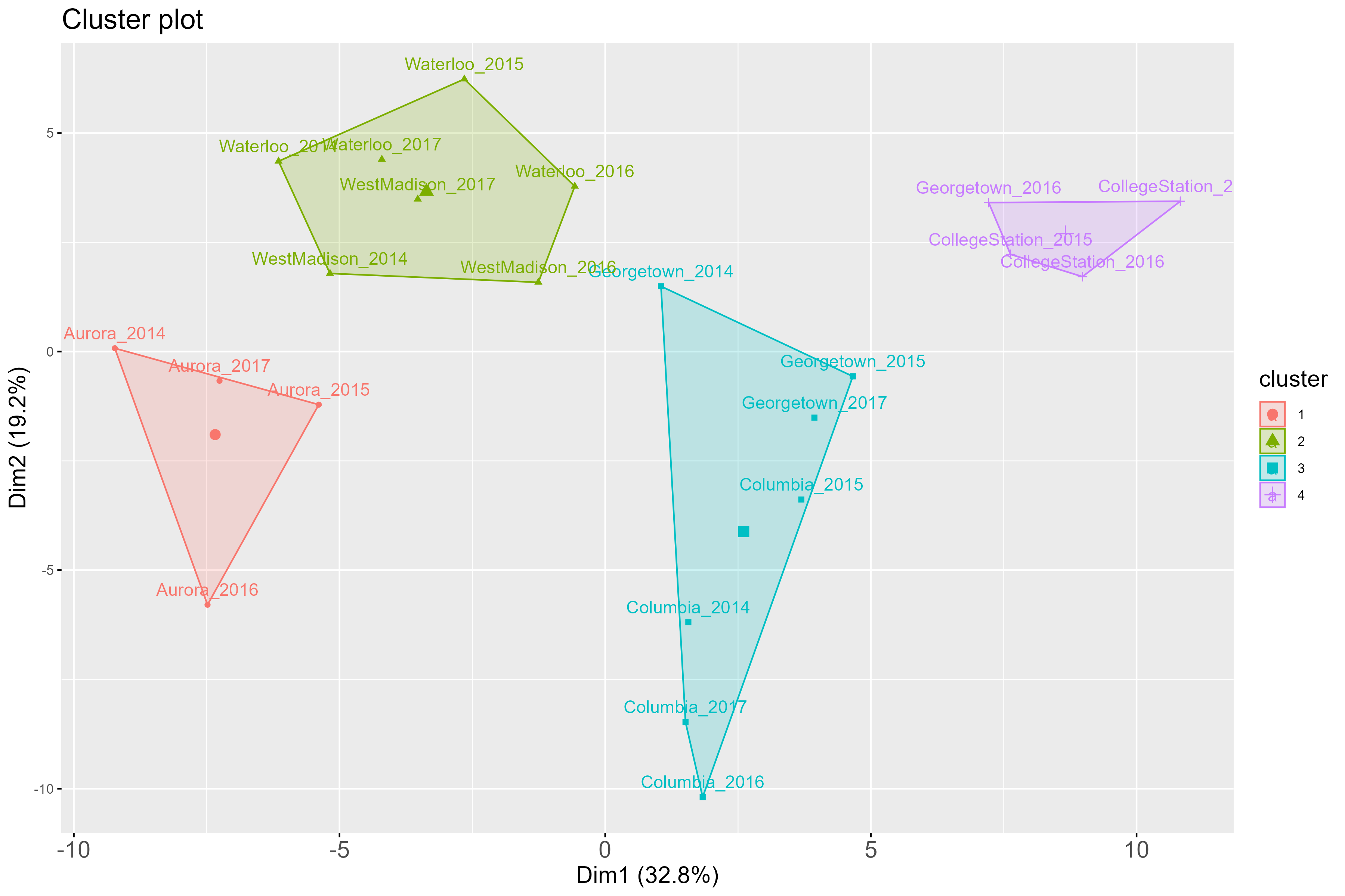
For instance, with k = 4,below is the plot of how environments included
in this MET dataset cluster, with k = 4:
Below is the plot obtained for the elbow method with different k values:
one should decide on the number of clusters so that, when adding another
cluster, it does not improve much the total intra-cluster variation
(that we want to minimize). In this case, 4 seems to be not so
bad!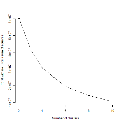
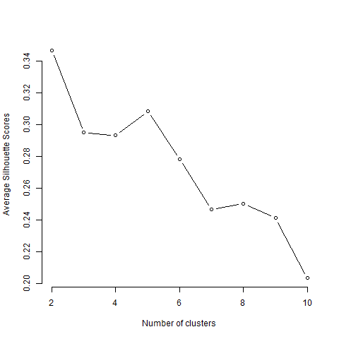
The Silhouette score is also used to validate results from clustering.
It gives a measure of how well observations are clustered with other
observations within a cluster. It is calculated for each observation of
the dataset, and the final metric corresponds to the average over all
observations for a given k. A large average Silhouette score reflects
that observations are well clustered with this k number of
clusters.
Here, 5 seems to be a better choice based on the Silhouette score.
Computing environmental covariates: different methods possible
In the first chunk of code presented above, daily weather data have
been saved in a folder called weather_data. We can load
these daily weather tables from NASA/POWER, and then implement different
methods to build day-windows (using the argument
method_ECs_intervals) which will represent climate variables
for the ML-based prediction models. To re-use the daily weather data
obtained via the NASA/POWER query, just specify these with the argument
raw_weather_data (see example below). These data will be
analyzed as
For instance with “fixed_length_time_windows_across_env” as below, with
day-windows computed in each environment with a width of 8 days:
Note: be careful to use a different path so that the clustering
analyses results obtained with the different environmental datasets do
not overlap!
daily_weather_tables_g2f <- readRDS("daily_weather_tables_nasapower.RDS")

METdata_G2F_2 <-
  learnMET::create_METData(
    geno = geno_G2F,
    pheno = pheno_G2F,
    map = map_G2F,
    climate_variables = NULL,
    compute_climatic_ECs = TRUE,
    raw_weather_data = daily_weather_tables_g2f,
    method_ECs_intervals = "fixed_length_time_windows_across_env",
    duration_time_window_days = 8,
    info_environments = info_environments_G2F,
    soil_variables = soil_G2F,
    path_to_save = '~/learnMET_analyses/G2F/method_2'
  )
## No climate covariates provided by the user.
## Computation of environmental covariates starts.
## Raw weather data are provided by the user and will be used to build environmental covariates.
## QC on daily weather data starts...
## QC on daily weather data is done!
## A file with flagged values has been saved in the subfolder weather_data.
## Computation of environmental covariates is done.
## Clustering of env. data starts.
## Clustering of env. data done.
## Soil and climate data will be included in the final METData object.
summary(METdata_G2F_2)
## object of class 'METData'
## --------------------------
## General information about the MET data
##
## No. of unique environments represented in the data: 22
##        unique years represented in the data: 4
##        unique locations represented in the data: 6
##
## Distribution of phenotypic observations according to year and location:
##
##        Aurora CollegeStation Columbia Georgetown Waterloo WestMadison
##   2014    212            236      244        224      181         200
##   2015    347            290      411        407      345           0
##   2016    228            197      328        227      207         303
##   2017    187              0      217        163      171         266
## No. of unique genotypes which are phenotyped
##  1913
## --------------------------
## Climate variables
## Weather data extracted from NASAPOWER for main weather variables?
## NO
## No. of climate variables available: 208
## --------------------------
## Soil variables
## No. of soil variables available: 4
## --------------------------
## Phenotypic data
##   No. of traits:  3
##
##      pltht         yld_bu_ac           earht
##  Min.   :117.2   Min.   :  2.814   Min.   : 48.0
##  1st Qu.:206.0   1st Qu.:114.641   1st Qu.:100.5
##  Median :232.5   Median :152.345   Median :115.6
##  Mean   :227.2   Mean   :147.758   Mean   :114.0
##  3rd Qu.:251.0   3rd Qu.:181.874   3rd Qu.:128.5
##  Max.   :351.0   Max.   :344.631   Max.   :195.0
##  NA's   :43                        NA's   :1072
## --------------------------
## Genotypic data
##   No. of markers : 106414
## --------------------------
## Map data
##   No. of chromosomes     10
##
##   markers per chromosome
##
##     1     2     3     4     5     6     7     8     9    10
## 16815 12533 11852  9507 13658  8151  8414  8936  8273  8275
If one has information about the phenological stages in each
environment (either by observations done from the field, or from results
from a crop growth model, for instance Sirius (Jamieson et al. (1998)) or APSIM (Keating et al. (2003), Holzworth
et al. (2014)), one can provide a table which
indicates at which day after planting the crop has reached a new
developmental stage. This table should be provided as input via the
argument intervals_growth_manual, and the method for computing
climate variables should now be chosen as
“user_defined_intervals”.
The names of each developmental stage can be indicated in the column
names, which can be useful after analyses to identify which wether-based
covariate had more weight in the machine learning model used. An example
of a table is given as example data in the package (see below).
The example provided is given to illustrate how the user should
format the table, but was not created to reflect the true growth stage
of the crop in these environments!
In this case, each growth period is estimated for all
genotypes tested in this environment: the package does not
incorporate at the moment specificity at the genotype level to take into
account genotypic variation regarding plant development and phenology.
For more information on this topic, please have a look at the following
publications: Heslot et al. (2014),
Technow et al. (2015), Rincent et
al. (2019).
| year | location | P | VE | V5 | V12 | R1 | R3 | R6 |
|---|---|---|---|---|---|---|---|---|
| 2014 | Aurora | 0 | 7 | 21 | 44 | 63 | 91 | 119 |
| 2014 | CollegeStation | 0 | 7 | 21 | 44 | 63 | 91 | 119 |
| 2014 | Columbia | 0 | 7 | 21 | 44 | 63 | 91 | 119 |
| 2014 | Georgetown | 0 | 7 | 21 | 44 | 63 | 91 | 119 |
| 2014 | Waterloo | 0 | 7 | 21 | 44 | 63 | 91 | 119 |
| 2014 | WestMadison | 0 | 7 | 21 | 44 | 63 | 91 | 119 |
One can also modify the base temperature (using the argument base_temperature - see example below) which is used to estimate accumulated GDD in each environment. The value of the base temperature depends on the crop under study and can be found in the literature (see https://en.wikipedia.org/wiki/Growing_degree-day#Baselines to get the base temperature for widely used crops).
METdata_G2F_2 <-
  learnMET::create_METData(
    geno = geno_G2F,
    pheno = pheno_G2F,
    map = map_G2F,
    climate_variables = NULL,
    compute_climatic_ECs = TRUE,
    raw_weather_data = daily_weather_tables_g2f,
    method_ECs_intervals = "user_defined_intervals",
    intervals_growth_manual = intervals_growth_manual_G2F,
    base_temperature = 12,
    info_environments = info_environments_G2F,
    soil_variables = soil_G2F,
    path_to_save = '~/learnMET_analyses/G2F/method_growth_stages'
  )
## No climate covariates provided by the user.
## Computation of environmental covariates starts.
## Raw weather data are provided by the user and will be used to build environmental covariates.
## QC on daily weather data starts...
## QC on daily weather data is done!
## A file with flagged values has been saved in the subfolder weather_data.
## Computation of environmental covariates is done.
## Clustering of env. data starts.
## Clustering of env. data done.
## Soil and climate data will be included in the final METData object.
Getting soil data from public database (SoilGrids)
If no soil data is provided by the user, it is possible to retrieve
publicly available data from the SoilGrids database (Poggio et al. (2021)). In this case, one needs to set
to TRUE the argument get_public_soil_data. In
this example, we use the multi-environment rice dataset deployed as a
toy dataset in learnMET (Monteverde et al. (2019)):
data("geno_indica")
data("map_indica")
data("pheno_indica")
data("info_environments_indica")
data("climate_variables_indica")

METdata_indica <-
    learnMET::create_METData(
        geno = geno_indica,
        pheno = pheno_indica,
        climate_variables = climate_variables_indica,
        compute_climatic_ECs = F,
        info_environments = info_environments_indica,
        map = map_indica,
        get_public_soil_data = T,
        path_to_save = "~/learnMET_analyses/indica_rice_data"
    )
## No soil covariates provided by the user.
## The package will retrieve soil data from the SoilGrids (ISRIC) Database.
## Clustering of env. data starts.
## Only one location used so no variance in the soil predictors. No clustering analyses possible.
## Clustering of env. data done.
## Soil and climate data will be included in the final METData object.

colnames(METdata_indica$env_data %>% dplyr::select(METdata_indica$list_soil_predictors))
##  [1] "silt_0-5cm"        "silt_5-15cm"       "silt_15-30cm"
##  [4] "silt_30-60cm"      "silt_60-100cm"     "clay_0-5cm"
##  [7] "clay_5-15cm"       "clay_15-30cm"      "clay_30-60cm"
## [10] "clay_60-100cm"     "sand_0-5cm"        "sand_5-15cm"
## [13] "sand_15-30cm"      "sand_30-60cm"      "sand_60-100cm"
## [16] "bdod_0-5cm"        "bdod_5-15cm"       "bdod_15-30cm"
## [19] "bdod_30-60cm"      "bdod_60-100cm"     "cec_0-5cm"
## [22] "cec_5-15cm"        "cec_15-30cm"       "cec_30-60cm"
## [25] "cec_60-100cm"      "nitrogen_0-5cm"    "nitrogen_5-15cm"
## [28] "nitrogen_15-30cm"  "nitrogen_30-60cm"  "nitrogen_60-100cm"
## [31] "phh2o_0-5cm"       "phh2o_5-15cm"      "phh2o_15-30cm"
## [34] "phh2o_30-60cm"     "phh2o_60-100cm"    "soc_0-5cm"
## [37] "soc_5-15cm"        "soc_15-30cm"       "soc_30-60cm"
## [40] "soc_60-100cm"