Evaluation of the model performance of a stacked model using CV0 on a rice dataset for phenotypic prediction
Cathy Westhues
2022-09-29
Source:vignettes/vignette_cv_stacking_indica.Rmd
vignette_cv_stacking_indica.RmdStep 1: Specifying input data and processing parameters
First, we create an object of class with the function create_METData().
The user must provide as input data genotypic and phenotypic data, as
well as basic information about the field experiments (e.g. longitude,
latitude data at least), and possibly environmental covariates (if
available). These input data are checked and warning messages are given
as output if the data are not correctly formatted.
In this example, we use an indica rice dataset from Monteverde et
al. (2019), which is implemented in the package as a “toy dataset”. From
this study, a multi-year dataset of rice trials containing phenotypic
data (four traits), genotypic and environmental data for a panel of
indica genotypes across three years in a single location is available
(more information on the datasets with
?pheno_indica,?geno_indica,?map_indica,?climate_variables_indica,?info_environments_indica).
In this case, environmental covariates by growth stage are directly
available and can be used in predictions. These data should be provided
as input in create_METData() using the argument
climate_variables. Hence, there is no need to retrieve with the
package any daily weather data (hence compute_climatic_ECs
argument set as FALSE).
Do not forget to indicate where the plots of clustering analyses should
be saved using the argument path_to_save.
library(learnMET)

data("geno_indica")
data("map_indica")
data("pheno_indica")
data("info_environments_indica")
data("climate_variables_indica")

METdata_indica <-
  learnMET::create_METData(
    geno = geno_indica,
    pheno = pheno_indica,
    climate_variables = climate_variables_indica,
    compute_climatic_ECs = F,
    info_environments = info_environments_indica,
    map = map_indica,
    path_to_save = '~/learnMET_analyses/indica/stacking'
  )
# No soil covariates provided by the user.
# Clustering of env. data starts.
# Clustering of env. data done.
The function print.summary.METData() gives an overview
of the MET data created.
summary(METdata_indica)
# object of class 'METData'
# --------------------------
# General information about the MET data
#
# No. of unique environments represented in the data: 3
#        unique years represented in the data: 3
#        unique locations represented in the data: 1
#
# Distribution of phenotypic observations according to year and location:
#
#        TreintayTres
#   2010          327
#   2011          327
#   2012          327
# No. of unique genotypes which are phenotyped
#  327
# --------------------------
# Climate variables
# Weather data extracted from NASAPOWER for main weather variables?
# NO
# No. of climate variables available: 54
# --------------------------
# Soil variables
# No. of soil variables available: 0
# --------------------------
# Phenotypic data
#    No. of traits:  3
#
#        GY             PHR               GC
#  Min.   : 6523   Min.   :0.4257   Min.   :0.00000
#  1st Qu.:10179   1st Qu.:0.5950   1st Qu.:0.02241
#  Median :10825   Median :0.6097   Median :0.03450
#  Mean   :10922   Mean   :0.6055   Mean   :0.03631
#  3rd Qu.:11605   3rd Qu.:0.6220   3rd Qu.:0.04752
#  Max.   :15388   Max.   :0.6816   Max.   :0.22306
# --------------------------
# Genotypic data
#    No. of markers : 92430
# --------------------------
# Map data
#    No. of chromosomes     12
#
#    markers per chromosome
#
#     1     2     3     4     5     6     7     8     9    10    11    12
# 11431 10435  8807 10943  5892  6326  5643  6365  7196  5390  8215  5787
Step 2: Cross-validated model evaluation
Specifying processing parameters and the type of prediction model
The goal of predict_trait_MET_cv() is to assess a given
prediction method using a certain type of cross-validation (CV) scenario
on the complete training set. The CV schemes covered by the package
correspond to those generally evaluated in related literature on MET
(Jarquı́n et al. (2014);
Jarquı́n et al. (2017);Costa-Neto,
Fritsche-Neto, and Crossa (2021)).
Here, we will use the CV0: predicting the performance of genotypes in
untested environment(s), i.e. no phenotypic observations from these
environment(s) included in the training set, and more specifically, the
leave-one-year-out scenario.
The function predict_trait_MET_cv() also allows to
specify a specific subset of environmental variables from the
METData$env_data object to be used in model fitting and predictions via
the argument list_env_predictors.
How does predict_trait_MET_cv() works?
When predict_trait_MET_cv() is executed, a list of
training/test splits is constructed according to the CV scheme chosen by
the user. Each training set in each sub-element of this list is
processed (e.g. standardization and removal of predictors with null
variance.
The function applies a nested CV to obtain an unbiased generalization
performance estimate, implying an inner loop CV nested in an outer CV.
The inner loop is used for model selection, i.e. hyperparameter tuning
with Bayesian optimization, while the outer loop is responsible for
evaluation of model performance. Additionnally, there is a possibility
for the user to specify a seed to allow reproducibility of analyses. If
not provided, a random one is generated and provided in the results
file.
In predict_trait_MET_cv(), predictive ability is always
calculated within the same environment (location–year combination),
regardless of how the test sets are defined according to the different
CV schemes.
Let’s use a meta-learner to predict a phenotypic trait!
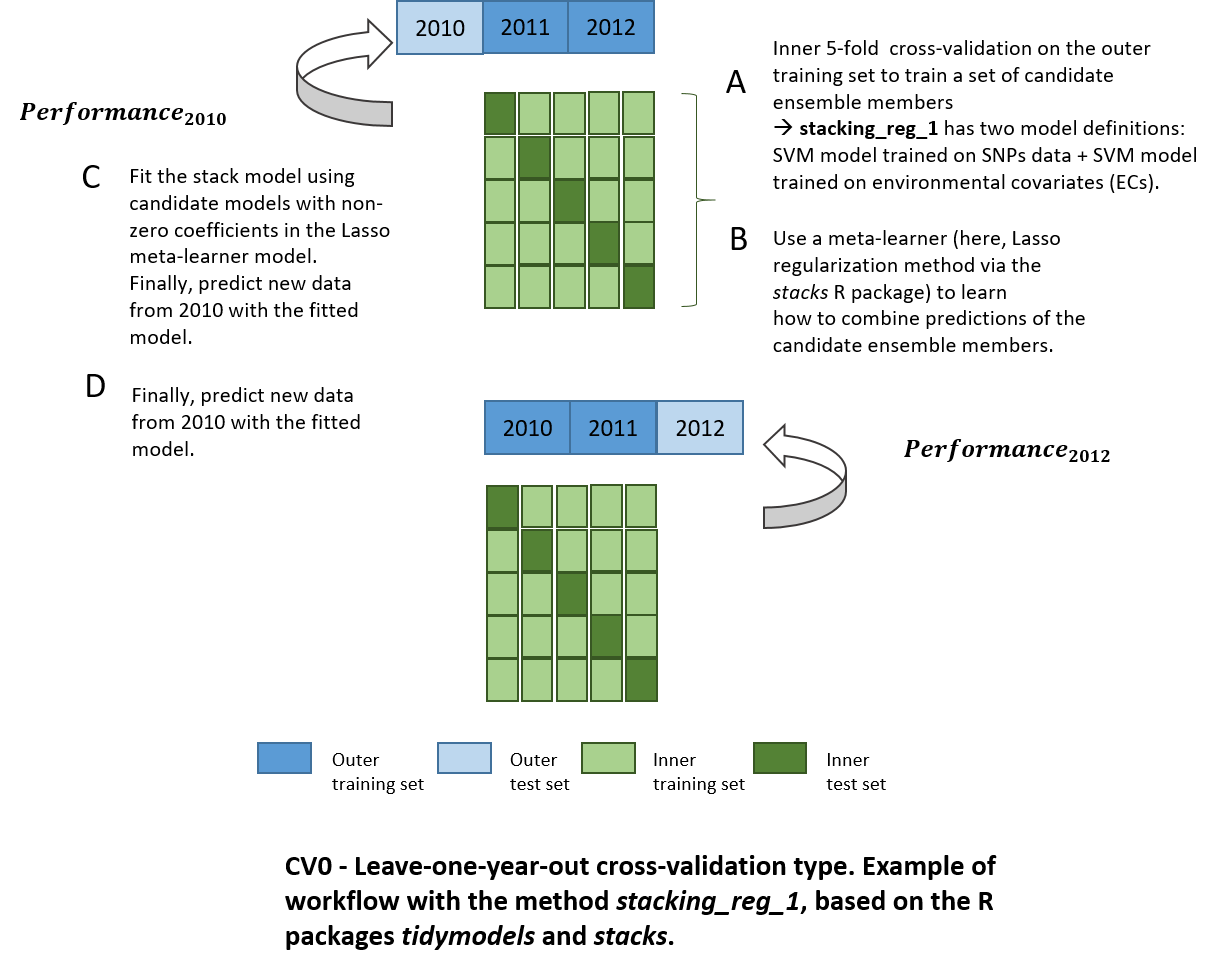
Model stacking corresponds to an ensemble method which exploits many
well-working models on a classification or regression task by learning
how to combine outputs of these base learners to create a new model.
Combined models can be very different: for instance, K-nearest
neighbors, support vector machines and random forest models, trained on
resamples with different hyperparameters can be used jointly in a
stacked generalization ensemble.
In the example below, we run a cross-validation of type CV0 with this method:
rescv0_1 <- predict_trait_MET_cv(
  METData = METdata_indica,
  trait = 'GC',
  prediction_method = 'stacking_reg_1',
  use_selected_markers = F,
  lat_lon_included = F,
  year_included = F,
  cv_type = 'cv0',
  cv0_type = 'leave-one-year-out',
  kernel_G = 'linear',
  include_env_predictors = T,
  save_processing  = T,
  seed = 100,
  path_folder = '~/INDICA/stacking/cv0'
)
Note that many methods for processing data based on user-defined parameters and machine learning-based methods are using functions from the tidymodels (https://www.tidymodels.org/) collection of R packages (Kuhn and Wickham (2020)). We use here in particular the package stacks (https://stacks.tidymodels.org/index.html), incorporated in the tidymodels framework to build these stacking models.
Extraction of results from the output
Let’s have a look now at the structure of the output rescv0_1.
The object of class list, met_cv contains 3 elements:
list_results_cv, seed_used and cv_type.
list_results_cv
The first element list_results_cv is a list of res_fitted_split
objects, and has a length equal to the number of training/test sets
partitions, which is determined by the cross-validation scenario.
Above, we ran predict_trait_MET_cv() with a
leave-one-year-out CV scheme, and the dataset contains three years of
observations. Therefore, we expect the length of to be equal to 3:
cat(length(rescv0_1$list_results_cv))
# 3
cat(class(rescv0_1$list_results_cv[[1]]))
# res_fitted_split
Within each of this res_fitted_split object, 9 elements are provided:
# prediction_method ; parameters_collection_G ; parameters_collection_E ; predictions_df ; cor_pred_obs ; rmse_pred_obs ; training ; test ; vipThe first sub-element precises which prediction method was called:
For example, to retrieve the data.frame containing predictions for the test set, we extract the predictions_df subelement (predictions in column named “.pred”):
predictions_year_2010 <- rescv0_1 $list_results_cv[[1]]$predictions_df
predictions_year_2011 <- rescv0_1 $list_results_cv[[2]]$predictions_df
predictions_year_2012 <- rescv0_1 $list_results_cv[[3]]$predictions_df
To directly look at the Pearson correlations between predicted and observed values for each environment, we extract the cor_pred_obs.
cor_year_2010 <- rescv0_1 $list_results_cv[[1]]$cor_pred_obs
cor_year_2011 <- rescv0_1 $list_results_cv[[2]]$cor_pred_obs
cor_year_2012 <- rescv0_1 $list_results_cv[[3]]$cor_pred_obs

head(cor_year_2010)
# # A tibble: 1 x 2
#   IDenv               COR
#   <chr>             <dbl>
# 1 TreintayTres_2010 0.340
head(cor_year_2011)
# # A tibble: 1 x 2
#   IDenv               COR
#   <chr>             <dbl>
# 1 TreintayTres_2011 0.399
head(cor_year_2012)
# # A tibble: 1 x 2
#   IDenv               COR
#   <chr>             <dbl>
# 1 TreintayTres_2012 0.372
To get the root mean square error between predicted and observed values for each environment, we extract the rmse_pred_obs.
rmse_year_2010 <- rescv0_1 $list_results_cv[[1]]$rmse_pred_obs
rmse_year_2011 <- rescv0_1 $list_results_cv[[2]]$rmse_pred_obs
rmse_year_2012 <- rescv0_1 $list_results_cv[[3]]$rmse_pred_obs
head(rmse_year_2010)
# [1] 1.583467
head(rmse_year_2011)
# [1] 2.490381
head(rmse_year_2012)
# [1] 2.314676
For a stacked prediction model, one can have a look at the coefficients assigned by the LASSO metalearner to the predictions obtained from the single base learners (here, support vector machine regression models) which respectively use genomic information:
head(rescv0_1 $list_results_cv[[3]]$parameters_collection_G)
#          member         cost      coef
# 1 svm_res_G_1_1 3.126802e-02        NA
# 2 svm_res_G_1_2 2.549168e+00        NA
# 3 svm_res_G_1_3 9.875661e-04 0.2918148
# 4 svm_res_G_1_4 3.368297e-01        NA
# 5 svm_res_G_1_5 1.382958e+01        NA
# 6 svm_res_G_1_6 6.927184e-03        NA
… and based on environmental information:
head(rescv0_1 $list_results_cv[[3]]$parameters_collection_E)
#          member        cost        sigma      coef
# 1 svm_res_E_1_1 0.648700227 2.924271e-08 0.0000000
# 2 svm_res_E_1_2 0.026507046 9.279021e-07 0.0000000
# 3 svm_res_E_1_3 2.398485546 7.941728e-08 0.0000000
# 4 svm_res_E_1_4 0.286690960 1.587980e-03 0.6687404
# 5 svm_res_E_1_5 0.007003367 5.721131e-01 0.0000000
# 6 svm_res_E_1_6 0.001157208 2.387000e-10 0.0000000
seed_used
To get the seed used for building the train/test partitions (especially useful for CV1 and CV2):
cat(rescv0_1 $seed_used)
# 100
cv_type
To get the type of CV used in the evaluation by
predict_trait_MET_cv():
cat(rescv0_1 $cv_type)
# cv0_leave-one-year-out